DuckDB Internals: Why is DuckDB Fast? (Part 2 Vectorized Execution)

DuckDB has become one of those rare pieces of software whose greatness is difficult to capture in words. Part of that is its versatility. It is approachable enough for anyone to install, point at a Parquet file, and begin exploring data on a laptop within minutes, yet sophisticated enough to support serious production systems and an entire ecosystem of companies and tools.

What makes DuckDB especially remarkable is how naturally its ease of use coexists with its technical depth. DuckDB is serious software built on decades of database research, yet DuckLabs, the team behind DuckDB, has somehow kept the project and its broader ecosystem lighthearted and fun.

Taking a look under the covers though reveals a great deal of careful engineering. Look up why is DuckDB fast and the first few search results often have fancy buzzwords like: in-process, columnar storage, vectorized execution, or parallel processing, but what does that actually mean?

Part 1 of this series followed a query from SQL text through parsing, binding, planning, optimization, and storage. This post picks up where that left off: execution.

More specifically, vectorized execution: how DuckDB processes data in batches instead of one row at a time.

Instructions per cycle

To understand why batching matters, you need a rough picture of what a CPU core can do.

A CPU core runs on a clock that ticks billions of times a second. A core running at 3 GHz experiences roughly 3 billion ticks each second. Instructions per cycle (IPC) then measures how many instructions the core can complete per tick on average. At 1 IPC it completes one per tick; at 3 IPC, three. IPC is not fixed though, it depends on both the processor and the software running on it.

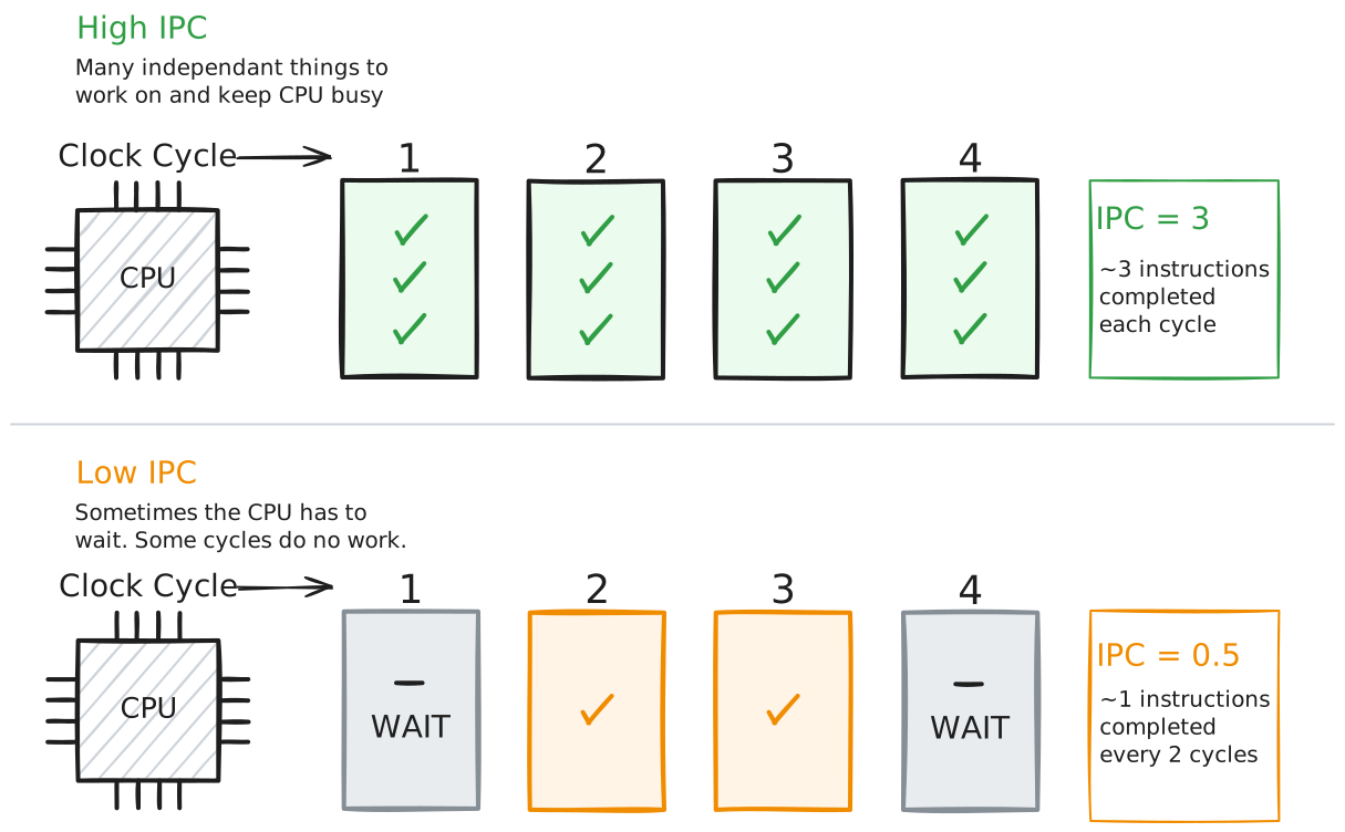
A CPU can complete more instructions per cycle when the software gives it several useful things to work on at once without frequently forcing it to pause. IPC can fall below one when the CPU has to wait. It could be waiting on data from memory or waiting for one instruction to produce a value the next one needs. An IPC below 1 means some cycles pass without any instruction completing at all.

In 2005, MonetDB/X100 measured how efficiently traditional databases were using the CPU. Running Query 1 in TPCH, MySQL's busiest routines, which operated one row at a time, sustained an IPC of 0.8. A single addition performed through MySQL took roughly 49 CPU cycles. X100, by contrast, could perform a similar operation in about 2.2 cycles by processing many values together in batches.

Much of that difference came from MySQL's query executor: the Volcano model.

The Volcano Model

For thirty years the Volcano model has been the standard way to build a query executor, and engines like PostgreSQL and MySQL are built on this exact model (SQLite is also row-at-a-time, though it does not use the Volcano model).

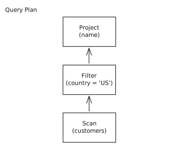
A query plan in Volcano is a tree of operators. Take a simple one:

SELECT 
    name 
FROM customers 
WHERE 
    country = 'US';

After planning, that becomes three operators: a scan at the bottom that reads rows, a filter that drops rows where country is not 'US', and a projection on top that keeps only name.

Every operator exposes the same three methods: open() to set up, next() to produce one row, and close() to clean up. The engine asks the top operator for a row by calling Project.next(). Project has no rows of its own, so it calls Filter.next(), which calls Scan.next(). The scan reads one row and passes it up. The filter checks the predicate and either passes the row along or discards it and asks the scan for another. Project trims the row to name and returns it. Then the engine asks for the next row and the whole chain runs again.

Data is pulled up through the tree, one row per request, which is why this is called pull-based execution. Every operator implements the same interface, so operators can stack on each other, and adding a new one means writing the same open/next/close contract.

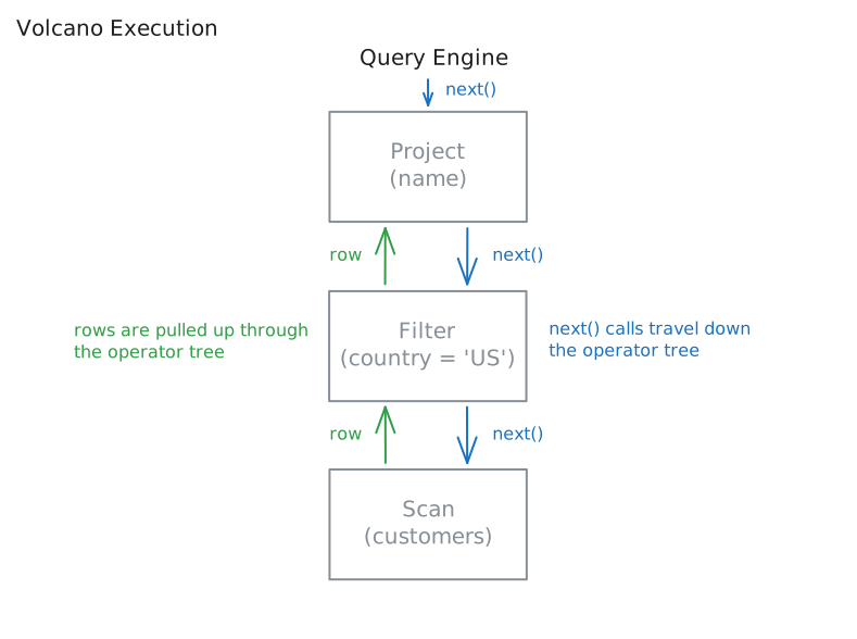
That flexibility comes with a cost. Each row has to travel through the entire chain of next() calls before work on the next row can begin. For a query that processes a million rows, each operator may be called a million times, which repeatedly pays the overhead of function calls, dispatch, etc.

Batches that fit in cache

MonetDB/X100 explored two ways to escape Volcano's per-row overhead.

The first was to operate on entire columns at once. Load all million values of country into memory, run the filter across the whole array in a tight loop, and pass the resulting array to the next operator. Instead of invoking an operator once per row, the engine invokes it once for the entire column.

This removes most of the per-row overhead, but introduces another problem. A million 8-byte values occupy 8 MB, which is too large for L1 and L2 cache. As each operator reads one large array and produces another, that data has to be moved repeatedly into and out of slower levels of memory, like RAM, and execution can be bottlenecked by memory bandwidth.

X100 proposed a middle ground: process data in batches, with each batch large enough to spread the cost of each operator call across many values, but small enough to remain cache-friendly.

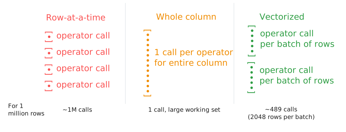
DuckDB commonly uses batches of 2048 rows. One operator call now covers 2048 rows, so the same million rows can be covered in about 489 calls instead of a million with Volcano.

This style of execution is called vectorized execution.

DataChunks and vectors

Data chunks and vectors are what DuckDB uses natively to store and represent data. For this reason, the data chunk interface is the most efficient way of interfacing with DuckDB.

A Vector represents the values from one column for a batch of rows. In DuckDB, a vector typically holds 2048 values—this number is configurable. For example, a flat Vector might contain up to 2048 values from amount_cents, stored as a contiguous array of 64-bit integers

A DataChunk represents a horizontal slice of a table, they hold a number of vectors, with every vector representing the same rows. In other words, it's a batch of rows laid out column by column.

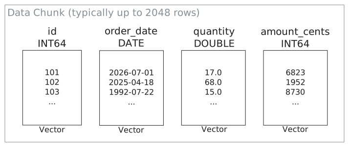
During execution, DuckDB passes DataChunks between operators. Each operator receives a chunk and works on the vectors it needs.

A filter on quantity, for example, reads the quantity Vector to determine which rows match. A projection calculating amount_cents * 2 reads that Vector and writes the results into a new one.

A DataChunk is not guaranteed to fit entirely in CPU cache. A wide chunk may contain many columns, and variable-length values such as string may refer to memory stored elsewhere. The important point is that DuckDB works on batches rather than entire columns. This keeps the working set relatively small, and an operator often needs to touch only a few of the vectors in the chunk.

Four Vector Types

Vectors logically represent arrays that contain data of a single type. The simplest way to store a vector is an array containing one value for every row. DuckDB calls this a flat vector.

But not every vector needs to store all of its values separately. DuckDB can support different vector formats that allow it to store the same logical data with a different physical representation. A column may contain the same value for every row, represent a predictable sequence, or simply refer to values stored in another vector. DuckDB has four core vector formats that let it use simpler vectors rather than immediately expanding everything into a flat vector.

Flat Vector

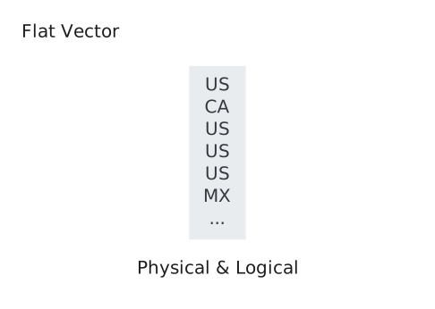
A flat vector stores its values in a contiguous array, this is the standard uncompressed representation of a vector. Its logical reprentation and physical representation are identical.

Constant Vector

A constant vector stores a single value that applies to every row.

DuckDB can use a constant vector for a literal such as the 2 in amount_cents * 2, since the value is identical across the entire batch, rather than store 2048 copies of 2.

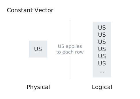
Constant vectors can also save computation. When every input to an expression is constant, DuckDB can evaluate the expression once and return another constant vector rather than repeating the same work for every row.

Dictionary Vector

A dictionary vector stores a child vector together with a selection vector. The selection vector contains indicies that say which position in the child represent each row.

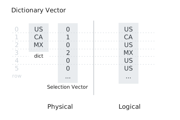
Suppose a filter keeps rows 0, 2, 4, and 5 from the vector above.

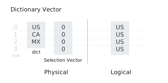
DuckDB can represent the filtered result by changing the selection vector rather than copying four strings into a new array.

Sequence Vector

A sequence vector represents values using a starting value and an increment.

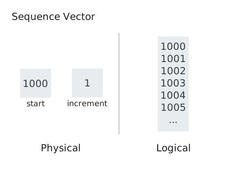
DuckDB commonly uses sequence vectors for row identifiers. The start and increment contain enough information to reconstruct any value in the vector, so there is no need to allocate and fill an array unless an operation requires the values in flat form.

Unified Vector Format

These four representations save storage and sometimes computation, but they create a problem for the functions that consume them.

Consider the following expression:

a + b

Each input could be flat, constant, dictionary, or sequence. Handling every pairing separately would require sixteen combinations for addition alone, before accounting for other operators and data types.

DuckDB avoids requiring a completely separate implementation for each combination through UnifiedVectorFormat. It gives generic vector code a common view containing three main pieces:

• a pointer to the underlying data
• a selection vector
• a validity mask

The selection vector tells the function which position in the underlying data belows to each logical row.

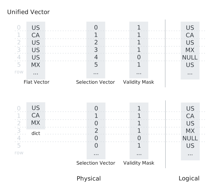
For the flat vector, the selection is simply [0, 1, 2, 3]. For the dictionary vector, it redirects each logical row to a position in the child.

Common vector pairings may not need to use the unified format. DuckDB can still use specialized paths where a representation makes an operation especially simple. A calculation involving only constants can be performed once, while operations over flat vectors can loop directly over their array.

Together, these representations allow DuckDB to delay copying or materializing values until an operation actually requires it.

Filters and selection vectors

The obvious way to return the result of a filter is to copy the resulting values into a new array. pandas works this way: df[df.x > 20] produces a new filtered dataframe. On a wide table that copying could be expensive, since the filter spends more time moving bytes than evaluating the predicate.

DuckDB can avoid that copy. A filter produces a selection vector: a list of the row indices that survived. Those indices point back into the vectors in the original DataChunk. The underlying arrays still contain all 2048 values, but subsequent work can operate only on the selected rows.

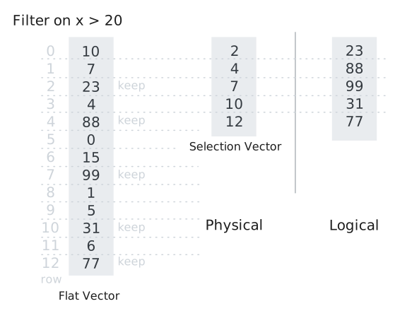
The selection vector is shared across the columns in the chunk. If row 7 survives because we filter on x = 99, row 7 is also the live row in every other vector in that DataChunk.

This is particularly important on wide data. A 50 column chunk passing through several predicates does not need to copy all 50 columns into a new buffer after each filter. The data can remain where it is while the selection vector carries the surviving row positions through the pipeline.

Vectors use another compact structure to track NULL values: the validity mask. It stores one bit per row, with 1 representing a value and 0 representing NULL.

Most vectors have no NULLs at all, so DuckDB does not need to allocate a validity mask for them. An absent mask means that every value is valid, allowing operators to skip per-row null checks.

Once DuckDB has resolved the vectors, the actual work often reduces to a small loop over the surviving values.

Inside the inner loop

The work up to this point has been about staging the data. The computation itself, comparing a value or adding two columns, happens in a small loop that walks the vectors one index at a time. This is the inner loop.

Take the query:

SELECT *
FROM lineitem
WHERE
    l_partkey = 42;

DuckDB may first use storage statistics to skip entire groups of data whose range cannot contain 42. It reads the remaining data in chunks, then runs the predicate over each l_partkey vector. The literal 42 is represented as a constant vector and the inner loop compares each value against it, recording matching rows in a selection vector.

Prebuilt loops

At this point, the remaining work looks simple: compare each l_partkey value with 42 and record the rows that match.

But the CPU cannot execute SQL directly. Somewhere, that comparison has to become machine instructions. Before DuckDB can compare a vector of int64 == int64, some compiled piece of code has to describe that comparison.

A database can produce that code in two broad ways.

Query compilation

One is to generate the code fresh for each query as it arrives. The database carries a compiler alongside its execution engine, translates the query plan into code specialized for that plan, and compiles it before execution begins. This is query compilation, often performed just-in-time (JIT).

HyPer is a well-known example of this approach. Because the generated code is built for one specific query, it can combine several steps into the same loop. A loop might filter a value, perform a calculation, and write the result without handing the row from one general purpose function to another.

Apache Spark uses a similar idea with whole-stage code generation. It takes several neighboring steps in a query plan and generates one larger piece of Java code for them. The JVM then compiles that code to JVM bytecode at runtime. Instead of repeatedly calling separate filter, projection, and join functions, Spark can perform much of that work inside the same loop.

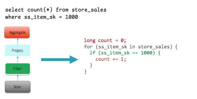
This can produce very efficient code, but it comes with a cost. The database must carry the machinery needed to generate and compile code while it is running. Compilation also adds some startup time before the query can begin.

Interpreted execution

DuckDB takes the other route. Instead of compiling each query, it interprets them. DuckDB contains a large collection of functions that were compiled when DuckDB itself was built. At runtime, it chooses the function that matches the operation and input types, then runs that function over the vector.

The loop for comparing int64 == int64 already exists inside the DuckDB binary. When DuckDB binds the expression:

l_partkey = 42

It determines that both sides are int64 values and connects the expression to the corresponding equality function.

This is called interpreted execution. DuckDB interprets the query plan by moving through its operators and calling the appropriate precompiled functions. duckdb_functions exposes a large catalog of functions, it's a useful approximation of choices available to the binder, although it's not a direct listing of every precompiled vector loop. During binding and execution, DuckDB selects one based on the operation and argument types.

D SELECT
     function_name,
     function_type,
     parameter_types,
     return_type
 FROM duckdb_functions()
 WHERE internal
   AND function_type IN ('scalar', 'aggregate')
 ORDER BY function_type, function_name
 LIMIT 1000;
┌───────────────────────┬───────────────┬─────────────────────────────────────┬───────────────────────┐
│     function_name     │ function_type │           parameter_types           │      return_type      │
│        varchar        │    varchar    │              varchar[]              │        varchar        │
├───────────────────────┼───────────────┼─────────────────────────────────────┼───────────────────────┤
│ any_value             │ aggregate     │ [DECIMAL]                           │ DECIMAL               │
│ any_value             │ aggregate     │ [ANY]                               │ ANY                   │
│ approx_count_distinct │ aggregate     │ [ANY]                               │ BIGINT                │
│ approx_quantile       │ aggregate     │ [DECIMAL, FLOAT]                    │ DECIMAL               │
│ approx_quantile       │ aggregate     │ [BIGINT, FLOAT]                     │ BIGINT                │
│ approx_quantile       │ aggregate     │ [TIMESTAMP, FLOAT]                  │ TIMESTAMP             │
│ approx_quantile       │ aggregate     │ [DOUBLE, FLOAT]                     │ DOUBLE                │
│ approx_quantile       │ aggregate     │ [DOUBLE, 'FLOAT[]']                 │ DOUBLE[]              │
│ approx_quantile       │ aggregate     │ [HUGEINT, 'FLOAT[]']                │ HUGEINT[]             │
│ approx_quantile       │ aggregate     │ [TIMESTAMP, 'FLOAT[]']              │ TIMESTAMP[]           │
│ approx_quantile       │ aggregate     │ [TIME, FLOAT]                       │ TIME                  │
│ approx_quantile       │ aggregate     │ [DECIMAL, 'FLOAT[]']                │ DECIMAL[]             │
│ approx_quantile       │ aggregate     │ [TINYINT, 'FLOAT[]']                │ TINYINT[]             │
│ approx_quantile       │ aggregate     │ [DATE, FLOAT]                       │ DATE                  │
│ approx_quantile       │ aggregate     │ [SMALLINT, FLOAT]                   │ SMALLINT              │
│ approx_quantile       │ aggregate     │ [SMALLINT, 'FLOAT[]']               │ SMALLINT[]            │
│ approx_quantile       │ aggregate     │ [INTEGER, FLOAT]                    │ INTEGER               │
│ approx_quantile       │ aggregate     │ [TIME WITH TIME ZONE, 'FLOAT[]']    │ TIME WITH TIME ZONE[] │
│ approx_quantile       │ aggregate     │ [BIGINT, 'FLOAT[]']                 │ BIGINT[]              │
│ approx_quantile       │ aggregate     │ [TIME WITH TIME ZONE, FLOAT]        │ TIME WITH TIME ZONE   │
│  ·                    │     ·         │   ·                                 │  ·                    │
│  ·                    │     ·         │   ·                                 │  ·                    │
│  ·                    │     ·         │   ·                                 │  ·                    │
│ min                   │ aggregate     │ [ANY]                               │ ANY                   │
│ min                   │ aggregate     │ [ANY, BIGINT]                       │ ANY[]                 │
│ min_by                │ aggregate     │ [BIGINT, DOUBLE]                    │ BIGINT                │
│ min_by                │ aggregate     │ [BIGINT, BIGINT]                    │ BIGINT                │
│ min_by                │ aggregate     │ [BIGINT, HUGEINT]                   │ BIGINT                │
│ min_by                │ aggregate     │ [INTEGER, BIGINT]                   │ INTEGER               │
│ min_by                │ aggregate     │ [INTEGER, HUGEINT]                  │ INTEGER               │
│ min_by                │ aggregate     │ [BIGINT, DATE]                      │ BIGINT                │
│ min_by                │ aggregate     │ [BIGINT, INTEGER]                   │ BIGINT                │
│ min_by                │ aggregate     │ [INTEGER, DOUBLE]                   │ INTEGER               │
│ min_by                │ aggregate     │ [DOUBLE, HUGEINT]                   │ DOUBLE                │
│ min_by                │ aggregate     │ [INTEGER, VARCHAR]                  │ INTEGER               │
│ min_by                │ aggregate     │ [INTEGER, DATE]                     │ INTEGER               │
│ min_by                │ aggregate     │ [INTEGER, TIMESTAMP WITH TIME ZONE] │ INTEGER               │
│ min_by                │ aggregate     │ [BIGINT, VARCHAR]                   │ BIGINT                │
│ min_by                │ aggregate     │ [INTEGER, INTEGER]                  │ INTEGER               │
│ min_by                │ aggregate     │ [INTEGER, TIMESTAMP]                │ INTEGER               │
│ min_by                │ aggregate     │ [DOUBLE, INTEGER]                   │ DOUBLE                │
│ min_by                │ aggregate     │ [BIGINT, TIMESTAMP]                 │ BIGINT                │
│ min_by                │ aggregate     │ [INTEGER, BLOB]                     │ INTEGER               │
└───────────────────────┴───────────────┴─────────────────────────────────────┴───────────────────────┘

The word interpreted can make this sound slow. DuckDB is not examining the SQL again for every value. By the time execution begins, the query has already been parsed, bound, planned, and connected to the functions it needs. Each function call then performs work over the whole vector, spreading the cost of that call across the 2048 rows.

Vectorization is what makes this approach practical. A function call would be expensive if it processed only one row, as in the Volcano model. When the same call processes an entire batch, its overhead is spread across the rows in that batch.

This also helps DuckDB remain easy to embed. It does not need to bundle a runtime compiler or initialize one before running queries. A JIT engine has to bundle one, often LLVM. That is a heavy dependency, and DuckDB is built to run embedded inside another process.

DuckDB therefore gives up some of the query-specific specialization available to a JIT engine. In return, it avoids compilation latency and carries less machinery.

The next question is how DuckDB keeps those general purpose loops cheap.

Keeping the loop cheap

One source of overhead is NULL. DuckDB stores a vector's data in one array and tracks which rows are NULL separately in a validity mask. The validity mask can represent the common case where every value is valid, meaning none of the values are NULL. When that is true, the inner loop can run directly over the data without performing a NULL check for each row.

When a mask may contain NULLs, DuckDB examines it in groups of 64. If all 64 are valid, it runs the operation across that group without checking the validity mask's rows individually. If none are valid, it can skip the entire group. Only a partially valid group requires checking the mask one bit at a time.

SIMD

For a predicate such as l_partkey = 42, the inner loop performs the same comparison for every value.

compare value 0 with 42
compare value 1 with 42
compare value 2 with 42
compare value 3 with 42

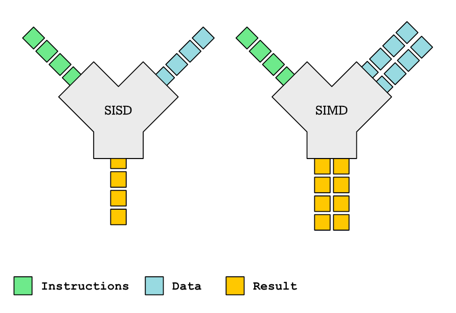
Some loops are simple enough for the C++ compiler to optimize when DuckDB itself is built. Instead of producing a separate CPU instruction for every comparison, the compiler may use SIMD instructions.

SIMD stands for single instruction, multiple data. It allows one CPU instruction to perform the same operation on a small group of values at once. The exact number of values processed together depends on the data type and the processor. It also does not happen for every operation. The compiler can only use SIMD when it can determine that the individual pieces of work are independent and can safely be performed together.

Push-based execution

In a pull-based engine, the consumer asks for data. The root operator asks its child for the next batch, that child asks its own child, and the request keeps moving downward until it reaches a scan. The resulting data then travels back up the tree.

Projection
↓ next()   ↑ row
Filter
↓ next()   ↑ row
Scan

Push-based execution flips this model. The executor starts at a source, obtains a batch, and pushes that batch through each operator until it reaches a sink. The producer side drives the pipeline.

Projection
↑ chunk
Filter
↑ chunk
Scan

DuckDB began as a pull-based engine, its original execution model was described as a Vector Volcano, a vectorized version of the Volcano model described earlier.

As DuckDB added more support for parallel execution, it later replaced that pull-based design with a push-based model. The problem was not about eliminating classic Volcano per-row overhead, vectorization had already spread that overhead across batches. The problem was that the pull-based model made parallel execution harder to express.

UNION ALL is a perfect example. In principle, its two inputs should be easy to process in parallel.

SELECT * FROM a 
UNION ALL 
SELECT * FROM b;

With one thread, the union can simply pull chunks from a until it's exhausted, then switch to b.

With multiple threads, the operator suddenly has to coordinate which worker pulls from which input: should it ask a, ask b, remember that a is finished, switch to b, or coordinate with other workers that might also be pulling from the same union?

Push-based execution makes the split explicit. Instead of repeatedly asking the union for another chunk, DuckDB can turn each input into a separate pipeline that can be scheduled independently.

Thread 1        Thread 2

Scan a          Scan b
   │               │
   ▼               ▼
      Shared Sink

One thread can scan chunks from a, another can scan chunks from b, and both can push their results into the same sink.

Under this model, every operator can take one of three roles:

1. A Source produces chunks, such as a table scan or the completed build side of a hash join when it is later scanned.
2. An Operator transforms a chunk into another chunk, like a filter or a projection.
3. A Sink consumes chunks and accumulates state. An aggregate may build a hash table, while an ORDER BY may collect rows into sorted groups.

A pipeline consists of one source, a chain of operators, and one sink.

Source → Operator → Operator → Sink

Each operator now holds only local state and has no idea what runs before or after it. That isolation is what makes the model useful for parallel execution. DuckDB can run several copies of a pipeline at once, split the input into pieces, and give each thread its own piece to process.

The operators in the middle can usually work independently on each chunk. The coordination instead happens at the source and sink. The source divides the input among the threads, while the sink combines their partial results.

This is also where parallel execution becomes more difficult. Sources may need to coordinate which thread receives each piece of input, while sinks may need to merge partial results, and the executor must determine when one pipeline can begin and another has finished.

Part 3 will follow that process.

At Greybeam, this is part of why building a multi-engine query router is so exciting for the future of data. It's clear that DuckDB is fast. DuckDB's strengths are real. So are Snowflake's. So are ClickHouse's.

We believe in a future where data teams can effortlessly use the query engine built to run each query the fastest. Come along for the ride.