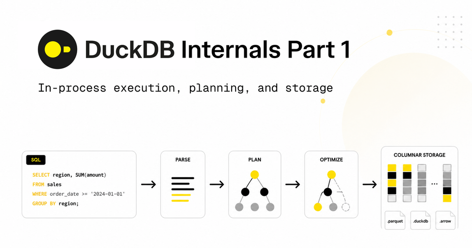
DuckDB Internals: Why is DuckDB Fast? (Part 1)

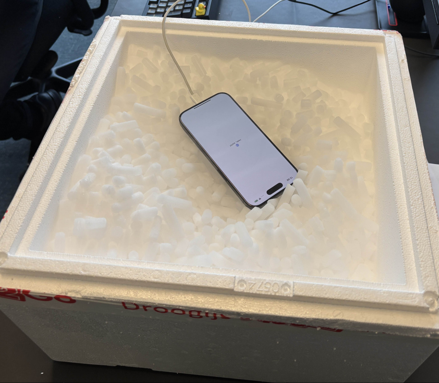
DuckDB has gone from a research project at CWI Amsterdam in 2019 to one of the most widely adopted databases of the past decade. The list of places it shows up is long: notebooks, ETL pipelines, dashboards, CI test runners, embedded analytics inside SaaS products, even an iPhone running TPC-H at scale factor 100.

Companies have started building real products around it. MotherDuck is wrapping DuckDB into a cloud data warehouse. BI and data app platforms like Hex, Omni, and Evidence use it as an in-app execution engine and cache. Fivetran's Managed Data Lake Service uses DuckDB inside its data-lake writer for merging and compaction. Rill builds an open-source BI tool on top of it. We use it at Greybeam too, powering millions of queries for BI and analytics workloads.

What is DuckDB?

DuckDB is an in-process analytical SQL database. Analytical means it's optimized for the kind of queries that scan millions of rows to filter, aggregate, and join — not the kind that look up a single record by primary key. In-process means there's no server. You don't connect to DuckDB; you load it as a library inside your program, the same way you'd load NumPy or Polars.

DuckDB has received widespread adoption because it's just so damn easy to use. It ships as a single binary under 20 MB with no external dependencies. You install it with pip install duckdb, brew install duckdb, or by linking libduckdb into a C++ project. It opens any directory of Parquet, CSV, or JSON files like they were already a SQL database.

DuckDB also happens to be one of the fastest single-node analytical engines available, regularly holding its own against entire clusters that cost millions of dollars per year.

This is the first post in a three-part deep dive into DuckDB internals. We'll follow a query from the moment it enters the engine to the moment the result is returned, and at each stage we'll look at the design choice that makes it fast.

DuckDB's speed comes from a handful design choices:

1. In-process execution
2. Columnar, compressed storage with zonemaps
3. Vectorized execution
4. Morsel-driven parallelism
5. Snapshot isolation with optimistic MVCC
6. And much more!

This post covers the path from your SQL to the moment the engine is ready to run the query, plus the storage layer the query will read from. By the end you'll have a clear mental model of DuckDB's setup work and storage layout. Query execution is covered in Part 2 so make sure to subscribe!

Queries Run In-Process

You point DuckDB at a 6 GB Parquet file on your laptop. The results come back in under a second. No cluster, no setup, no migration, no CREATE TABLE. How does that work?

SELECT
  *
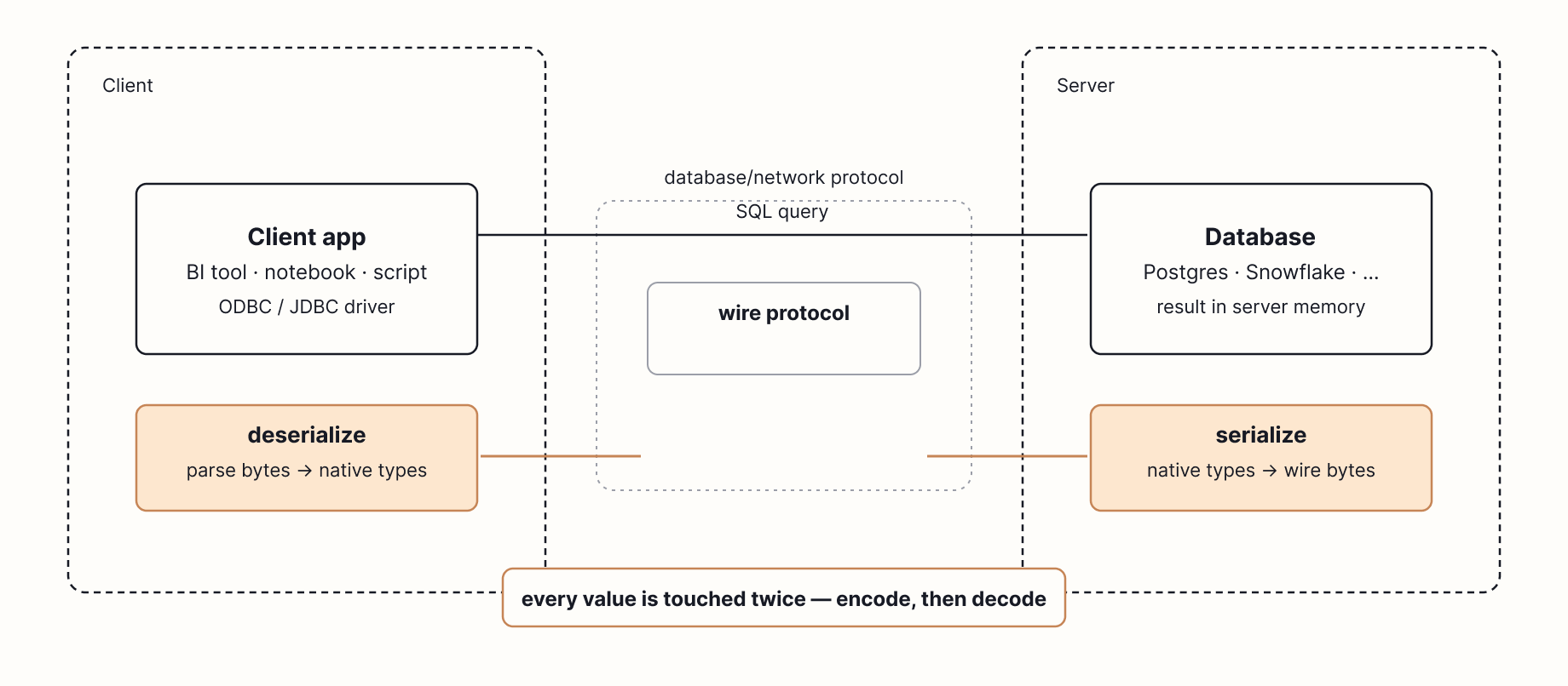
FROM 'orders.parquet';

Most analytical databases are servers. Snowflake, Postgres, BigQuery, Redshift. You open a connection, send SQL over TCP (a protocol to send data over a network), and wait for results to come back. Along the way, every record in the result is serialized into a wire protocol, transmitted across the network, and deserialized on the other end.

Serializing and Deserializing

Inside a database, a query result lives as typed values at specific memory addresses. A 64-bit integer here, a pointer to a string there. Those addresses only exist in that process. To send the result to a client on another machine, the database has to rewrite every value into an agreed byte format (Postgres has its own, MySQL has another, with ODBC and JDBC as client-side APIs that drivers expose on top) so it can be pushed through a TCP socket. The client then parses those bytes back into its own native types. Every value may be touched multiple times, once to encode and once to decode, and on a large result set, that work often takes longer than the query itself.

DuckDB is not a server. It's a library. There is no DuckDB daemon, no port, no cluster. You load libduckdb into your program and call functions directly against it.

In 2017, Mark Raasveldt and Hannes Mühleisen published Don't Hold My Data Hostage, a paper measuring what actually happens when you pull a result set out of a warehouse. They found that the client protocol itself — ODBC, JDBC, and similar row-by-row value APIs — was often the slowest single step in the entire query, sometimes dwarfing the time the database spent computing the answer.

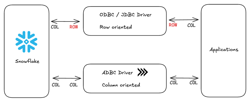
Two costs drive this. The first is raw bandwidth: a typical gigabit Ethernet link caps you at around 125 MB/s, and a large result set can take longer to transmit than it took to compute. The second is per-value overhead. ODBC and JDBC hand back results one row and one value at a time, which means the client makes a separate function call for every field in every row. On a 100-million-row result, that's hundreds of millions of function calls, each one doing its own little memory copy, type check, and string allocation.

ADBC transfers data between systems in columnar Arrow format, which avoids the row-by-row serialization/deserialization that ODBC and JDBC require. Our friends at Columnar are making this commonplace.

DuckDB sidesteps both bottlenecks by living in the same process as the client.

When a Python script runs con.sql("SELECT ... FROM my_df") against a pandas dataframe, DuckDB can use a feature called a replacement scan. Instead of copying the dataframe into an internal table first, DuckDB replaces the table reference with a function that reads from the dataframe when the query runs.

In the best case, DuckDB can read the same underlying buffers the Python process already owns, so it avoids materializing a second full copy of the data. This is zero-copy! If NumPy says "here's a buffer (contiguous chunk of memory) of 1 million int64 values," DuckDB can often read that same buffer directly because it understands the same physical layout.

In practice, whether the path is truly zero-copy depends on the dataframe’s physical layout, column types, null representation, and string storage. If the types or layouts do not line up, DuckDB may allocate converted buffers for some columns.

Arrow is the cleanest version of this story because Arrow is already a columnar, typed memory format designed for sharing data between systems. That is why returning DuckDB results as Arrow, or querying Arrow-backed data, can avoid much of the row-by-row conversion overhead that traditional APIs impose.

From SQL to Logical Plan

Once your SQL reaches DuckDB, it goes through the usual stages: parse, bind, plan, optimize.

Parsing

The first step is to parse SQL into an abstract syntax tree (AST). DuckDB uses a fork of the Postgres parser, which is part of why DuckDB's dialect feels so familiar.

An AST is a tree representation of your query where each node is a syntactic construct: a SELECT statement, a column reference, a function call, a join, a literal. Parsing turns the flat string SELECT sum(l_quantity) FROM lineitem WHERE l_shipdate > '2024-01-01' into a structured object the engine can actually reason about.

Select(
    expressions=[
        Sum(
            this=Column(
                this=Identifier(this=l_quantity, quoted=False)))],
    from_=From(
        this=Table(
            this=Identifier(this=lineitem, quoted=False))),
    where=Where(
        this=GT(
            this=Column(
                this=Identifier(this=l_shipdate, quoted=False)),
        expression=Literal(this='2024-01-01', is_string=True))))

A tree structure is what lets the rest of the engine do its job. The binder walks the nodes to resolve l_quantity to a specific column in a specific table. The optimizer pattern-matches subtrees to recognize that the WHERE predicate can be pushed down into the scan. The physical planner maps function call nodes to executable operators. None of these passes can operate on raw SQL. They need to traverse, pattern-match, and rewrite a typed structure.

Binding

The next step is binding, which resolves every name in the AST against the catalog. lineitem becomes a specific table with a known schema. l_quantity becomes a specific column with a known type. sum becomes a specific aggregate function whose input type matches that column. Type checking happens here too: comparing l_shipdate to the string '2024-01-01' works because the binder coerces the literal to a date.

The output is a bound tree where every node knows what it refers to and what type it produces. Errors like unresolved columns, ambiguous references, and type mismatches surface at this stage.

At this point, DuckDB has turned raw SQL text into a typed tree. The engine no longer sees l_quantity as just a string in a query; it sees a specific column with a specific type from a specific table.

The Optimizer

In DuckDB, the optimizer consists of a sequence of small, focused transformations that you can, in fact, inspect and disable individually.

D SELECT * FROM duckdb_optimizers();
┌────────────────────────────┐
│            name            │
│          varchar           │
├────────────────────────────┤
│ expression_rewriter        │
│ filter_pullup              │
│ filter_pushdown            │
│ empty_result_pullup        │
│ cte_filter_pusher          │
│ regex_range                │
│ in_clause                  │
│ join_order                 │
│ deliminator                │
│ unnest_rewriter            │
│ unused_columns             │
│ statistics_propagation     │
│ common_subexpressions      │
│ common_aggregate           │
│ column_lifetime            │
│ limit_pushdown             │
│ row_group_pruner           │
│ top_n                      │
│ top_n_window_elimination   │
│ build_side_probe_side      │
│ compressed_materialization │
│ duplicate_groups           │
│ reorder_filter             │
│ sampling_pushdown          │
│ join_filter_pushdown       │
│ extension                  │
│ materialized_cte           │
│ sum_rewriter               │
│ late_materialization       │
│ cte_inlining               │
│ common_subplan             │
│ join_elimination           │
│ window_self_join           │
└────────────────────────────┘
           33 rows          

Running SET disabled_optimizers = 'filter_pullup, join_order' turns specific passes off so you can see what they were doing.

Here are a few interesting optimizers:

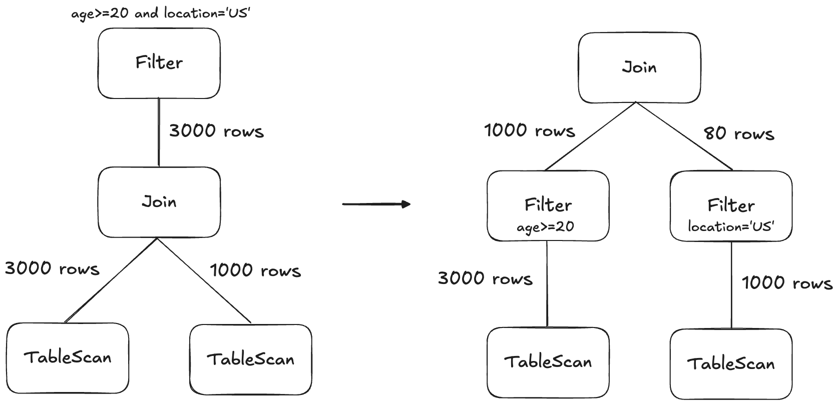
Filter pushdown

This is a classic database optimization: move WHERE predicates as close to the scan as possible so you prune data as early as possible. DuckDB first pulls filters up to the top of the plan so they can be combined and reorganized, then pushes them back down as far as possible.

Subquery unnesting

Correlated subqueries traditionally force a database to run the inner query once per outer row, which is slow. DuckDB implements techniques from the Unnesting Arbitrary Queries paper to rewrite these as joins, which are dramatically faster.

Dynamic join-filter pushdown

During a hash join (more on hash joins here), the build side has to be fully read before the probe side starts. DuckDB takes advantage of that ordering: once the build side is in memory, it computes the min and max of the join key values it actually contains, then pushes those bounds back into the probe-side scan as a runtime filter. If the build side turned out to contain values only between 100 and 200, the probe scan can use the table's zonemaps to skip any row groups outside that range before reading them.

When the build side has fewer than 50 distinct join key values, the filter becomes an IN list instead of a min-max range, which is more precise and skips even more rows.

Join order optimization

Join order is the most consequential decision the optimizer makes. The order in which joins run determines how big each intermediate result is. A query joining six tables has 30,240 possible tree shapes, and the difference between best and worst can be orders of magnitude in runtime. Picking well requires estimating how many rows each candidate join will produce, which depends on table sizes, predicate selectivity, and the order of joins that came before.

DuckDB models the query as a graph. Each table is a node, and each join predicate is an edge connecting the tables it references. The optimizer's job is to pick an order to combine the nodes into a single tree, where each combination is a join. For example, if we have a query joining a to b , b to c, and c to d, the graph might look like this:

a ── b ── c ── d

To find the best tree, DuckDB uses dynamic programming, such as DPhyp or DPccp. Dynamic programming is a fancy name for a simple idea: if you've already figured out the best way to join {a, b, c}, you can reuse that answer when figuring out the best way to join {a, b, c, d}. You don't need to re-explore all the orderings inside {a, b, c} . It does this for every connected pair, then triplet, then quadruplet, etc.

There are dozens more optimizations to explore and the entire optimization phase usually finishes in about a millisecond. After optimization, DuckDB has a logical plan. The next step is to translate that plan into something the engine can actually execute.

If you've enjoyed reading this so far, consider subscribing. We'll continue sharing more about the intricacies of DuckDB and many other query engines.

The Physical Plan

Imagine the optimizer hands the engine this plan, written in plain English:

Read events from disk. Drop the rows where event_date is on or before 2026-01-01. Group what's left by customer_id and add up amount. Sort the result by total descending. Return the top 10.

The engine now has to decide how to actually run those steps in a way that uses the CPU well and parallelizes across cores.

Mapping Logical Steps to Physical Operators

The optimizer's output is still a logical plan. It says what each step needs to compute but not which algorithm should do the computing. Most logical steps have several physical implementations.

Take a join. The same logical join can be turned into any of: hash join, index join, piecewise merge join, cartesian join.

DuckDB walks the logical plan and picks a physical operator for each node based on the shape of its inputs and predicates. The output is a physical plan — a tree of physical operators the executor knows how to run.

We will save the details of vectorized execution for Part 2, but one execution concept is useful now: the physical plan is not run as one giant tree walk. DuckDB breaks it into pipelines.

Pipelines

Think of a pipeline as an assembly line. Data enters at one end and passes through a chain of stations. Each station does one thing (drop a row, transform a column, look up a value in a hash table) and hands the result to the next station. As long as each station can decide what to do with a row using only that row, the line keeps moving. Examples of pipelines:

• WHERE: it either passes the row through or drops it. No state needed.
• A Projection: it computes new column values and emits them.
• Probe side of hash join: once the hash table has been built, it looks up the row's key in the hash table and emits the joined row or nothing if no match.

In DuckDB, a connected chain of streaming stations like this is called a pipeline. Pipelines parallelize cleanly since every CPU core can run its own copy of the assembly line on its own slice of the input.

Pipeline breakers

Some operators can't work this way. They need to see the entire input before they can produce an output.

• ORDER BY can't emit a single sorted row until its seen every row because it doesn't know which row belongs first.
• GROUP BY can't emit the final sum until it has accounted for every row in a grouping.
• Build side of a hash join has to build the hash table before it can start looking anything up.

These operators are called pipeline breakers or sinks. They mark the end of one pipeline and the beginning of the next. The physical plan is effectively a sequence of pipelines stitched together by sinks.

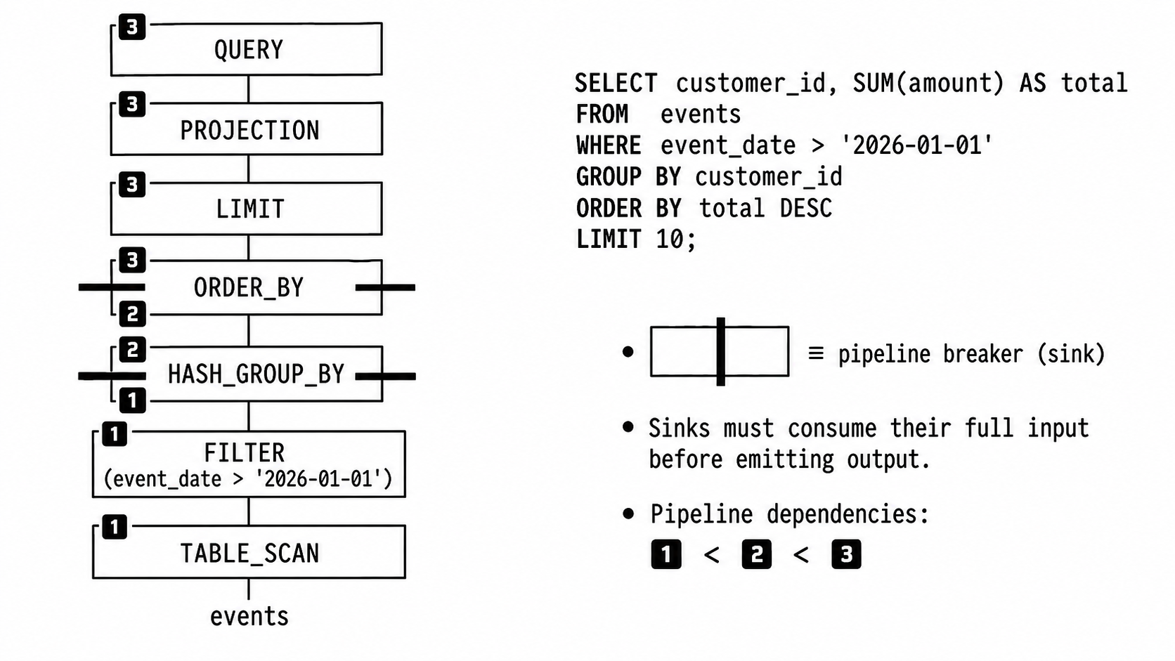
Going back to our original query, the physical plan may look something like this:

• Pipeline 1: ends at the GROUP BY sink:
  scan events → filter event_date > '2026-01-01' → write into GROUP BY's hash table
• Pipeline 2: ends at the ORDER BY sink:
  read groups out of the hash table → write them into the sorted run
• Pipeline 3: the final assembly line:
  read sorted runs → take the first 10 rows → return results

Each pipeline runs in parallel internally. Multiple threads run the entire assembly line at once, each on its own morsel of input. Pipelines that depend on each other run in sequence, because pipeline 2 can't start reading until pipeline 1's GROUP BY is done writing.

What Happens in a Sink

A sink runs in three phases: sink, combine, and finalize.

Sink

Every thread accepts chunks (DuckDB's 2048 row batches) and writes them into its own local state, for example, its own hash table for a HASH_GROUP_BY, its own sorted run for ORDER_BY, its own partial aggregate for UNGROUPED_AGGREGATE, its own hash table for the build side of HASH_JOIN. Threads do not share state. If every thread wrote into one shared hash table, they'd be fighting for a lock on every insert. Local state lets each thread sink at full speed with no coordination.

Combine

Once every thread finishes writing to its local space, the results have to merge into a single global state. For a GROUP BY, that means combining the partial sums and counts for each group across all the thread-local hash tables. DuckDB designs the sink so the combine step itself runs across all cores, rather than as a single-threaded merge at the end (covered in Part 3).

Finalize

The merged global state is read out as the input to the next pipeline. For our GROUP BY, that'll be a stream of customer_id, total) rows.

Parallelism is Local

A pipeline runs across all cores by giving each thread its own morsel of input. A sink runs across all cores by giving each thread its own local state and merging in parallel. DuckDB does not try to plan global parallelism for the whole query, it parallelizes one pipeline at a time. This is a part of what makes morsel-driven parallelism (covered in Part 3) and vectorized execution (covered in Part 2) work.

The Storage Layer

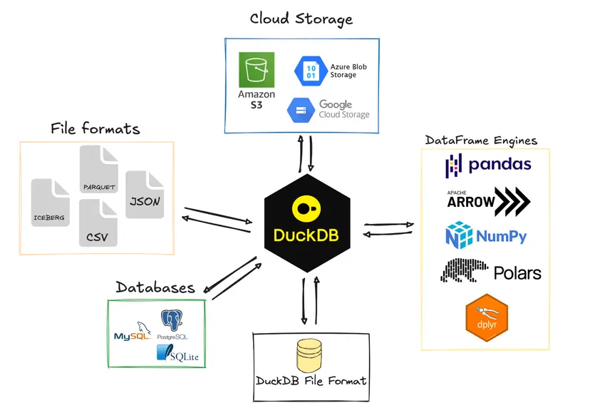
The amazing thing about DuckDB is that it can turn most files into a SQL database, and in fact is often used to directly query file formats like Parquet, CSV, JSON, XLSX, etc.

DuckDB database

A DuckDB database is a single file, conventionally .duckdb or .db. This was inspired by SQLite. One file is easy to move, backup, and share.

Inside the file, data is broken into fixed-size blocks. The default block size is 256 KB, though smaller block sizes (down to 16 KB) can be configured. The headers contain metadata like magic bytes, storage format versions, database headers, etc.

Every block also carries a checksum, a small value computed from the block's contents. When DuckDB reads a block, it recomputes the checksum and compares. If the values don't match, the data has been corrupted somehow, and DuckDB raises an error. Checksums are important because bits occasionally flip in memory or on disk: a cosmic ray hits a cell, a firmware bug drops a byte, a flaky cable corrupts a write, etc. Cloud data warehouses can mitigate this with built-in error correction in memory and redundancy across disks. Consumer hardware like laptops or edge devices generally have less protection, so checksumming is a useful backstop.

Columns, row groups, zone maps

Inside the blocks, columns are stored separately from each other. A row store keeps entire records contiguous on disk. For example:

[id_1, name_1, age_1]
[id_2, name_2, age_2]
[id_3, name_3, age_3]

This is fast for queries like SELECT * FROM users WHERE id = 42, because the record's bytes sit close together physically in memory.

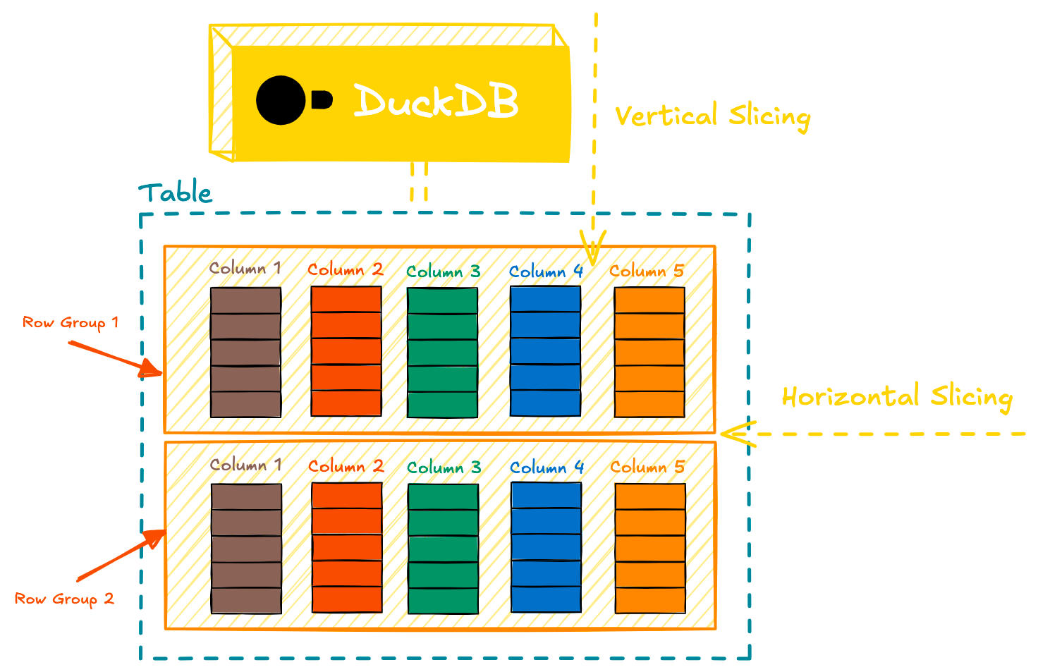
Column stores keep columns contiguous on disk.

[id_1, id_2, id_3]
[name_1, name_2, name_3]
[age_1, age_2, age_3]

A query that reads 4 columns from a 300 column table only needs to read those 4 columns. On a row store, all 300 columns would be read and 296 of those will need to be discarded. This is why organizations use column stores (Snowflake, BigQuery, ClickHouse, etc.) for analytics: queries tend to be selective, group on, and aggregate a few columns.

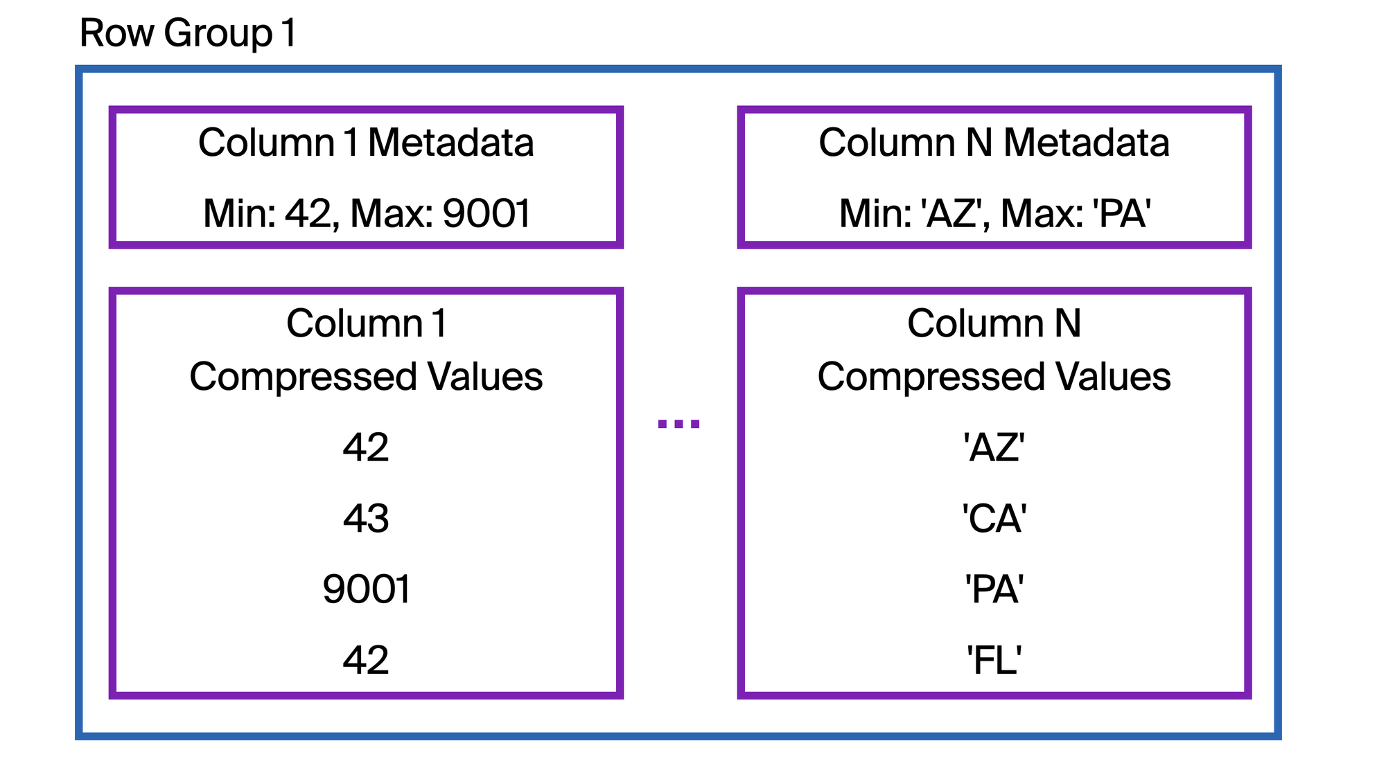
Row Groups

Each column is split into row groups of up to 122,880 rows, and within a row group, into column segments that typically map to a single 256 KB block. A row group is a unit of parallelism. A query running on 8 threads should have at least 8 row groups in scope to keep every thread busy.

Zone Maps

Each row group also carries a zone map. A zone map contains the min and max values in a row group, plus a null count. When a scan runs with a predicate like WHERE event_date > '2026-01-01', DuckDB checks each row group's max value before reading in any of its data. Row groups whose max event_date is on or before '2026-01-01' are skipped entirely.

This a similar technique major cloud data warehouses use, just under different names. Snowflake calls it micro-partition pruning, BigQuery calls it block pruning, ClickHouse uses minmax data skipping indexes.

Zone map effectiveness depends heavily on column ordering. A column that's sorted or naturally ordered by an insert timestamp gives narrow min-max spans per row group. A column whose values are scattered randomly across the table gives spans that cover wide ranges, and the zonemap is much less effective.

Parquet

Most of the time, practitioners aren't querying DuckDB tables. They're pointing DuckDB at Parquet files. There are two common patterns:

-- Query a parquet file directly
SELECT
  customer_id
  , SUM(amount) as total_amount
FROM read_parquet('/my/nice/files/*.parquet', union_by_name=TRUE)
WHERE
  event_date > '2026-01-01'
GROUP BY ALL;

-- Or load it into a DuckDB table first
CREATE TABLE events AS
SELECT * FROM read_parquet('s3://bucket/events/*.parquet');

Why is querying Parquet files so fast? DuckDB hasn't converted the data into its own format. There's no zone map built by DuckDB, no DuckDB-side compression, no .duckdb file. And yet, some queries run roughly as fast as a native DuckDB table.

Parquet has similar design principles as DuckDB's native format:

• Parquet is columnar. Each column lives in its own column chunk inside a row group. DuckDB reads only the column chunks the query references.
• Parquet stores min/max statistics per row group per column. DuckDB uses those same statistics exactly the way it uses zone maps.

When querying Parquet, DuckDB reads the footer to discover the file's schema and row group statistics. It uses those statistics to determine which row groups can satisfy query predicates. For each surviving row group, it reads only the column chunks the query needs, decompresses them, and feeds them into the pipeline-and-sink we described earlier.

When a file is stored remotely, DuckDB doesn't download the whole file. It issues an HTTP request to fetch just the footer, decides which row groups and column chunks it needs, then issues requests to fetch only those bytes. A WHERE clause that prunes properly can dramatically increase performance over the wire.

CSVs

CSV is the opposite of Parquet, it's not self-describing. Parquet effectively hands DuckDB a schema, statistics, chunked columns with compressed data. CSVs don't. They're just text. DuckDB needs to figure out what character separates columns, are values quoted, how are quotes escaped, does the first row contain column names, and what type each column should be. DuckDB does this with its CSV sniffer.

SELECT *
FROM 'events.csv';

-- Alternatively
SELECT *
FROM read_csv('events.csv');

When DuckDB reads a CSV, it automatically tries to detect three main things: the dialect, the column types, and whether the file has a header row.

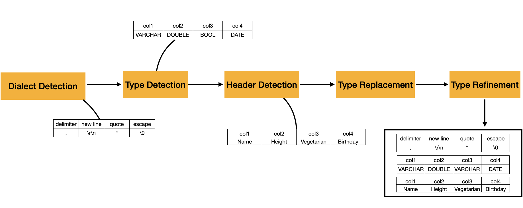
Dialect Detection

The dialect is the file’s parsing grammar: delimiter, quote character, escape character, and newline style. DuckDB tests candidate dialects and chooses the one that produces the most consistent rows and the highest number of columns. For example, a file like this:

Company|Category|City|IsSuperCool
DuckDB|OLAP database|Amsterdam, Netherlands|True
Snowflake|data warehouse|Bozeman, MT|True
BigQuery|data warehouse|Mountain View, CA|N/A
Greybeam|multi-engine router|San Francisco, CA|True

Should be split on |, not ,, even though the city names contain commas. The sniffer can figure that out because | produces a consistent four-column table.

Column Types

After the dialect is chosen, DuckDB detects column types by trying to convert sampled values in each column to candidate types. If a value cannot be converted to a candidate type, that type is removed from the candidate set for that column. After the samples are processed, DuckDB chooses the remaining candidate type with the highest priority. The documented default candidate types, in priority order, are NULL, BOOLEAN, TIME, DATE, TIMESTAMP, TIMESTAMPTZ, BIGINT, DOUBLE, and VARCHAR. Since every value can be represented as VARCHAR, it is the fallback type.

Headers

Header detection comes next. If the first row looks different from the rows below it, for example, strings like Company and Category are treated as the column names. Otherwise it generates default names like column0, column1, etc.

The sniffer works from a sample rather than scanning the full file. The default sample size is 20,480 rows. You can increase this, or set sample_size = -1 to inspect the whole file.

Execution

Clearly a lot of work happens before a query actually runs. It gets parsed into an AST, bound to the schema, optimized through ~30 passes, and compiled into a physical plan. Even the storage layer does so much work in advance.

Part 2 picks up at execution. Stay tuned!

At Greybeam, this is part of why building a multi-engine router is so exciting for the future of data. It's clear that DuckDB is fast. DuckDB's strengths are real. So are Snowflake's. So are BigQuery's.

We believe in a future where data teams can use the query engine built to run each query the fastest. Come along for the ride.